Tutorial: Güngören Landslide Analysis - Complete Workflow
Warning:
This tutorial and InSARLite are provided for research and educational use only. Validate all results with independent data and do not use outputs for safety critical or operational decision-making.
InSARLite is built on GMTSAR and uses it to run the processing steps. Therefore, GMTSAR assumptions, limitations, and any known issues or bugs may also affect InSARLite outputs.
InSAR processing may require substantial CPU time, RAM, and disk space. Please ensure you have adequate computing infrastructure (please see prerequisites below) before starting, otherwise processing may be slow or may fail.
Introduction
This tutorial demonstrates the complete InSARLite workflow using a case study area where a fatal landslide occurred in northeastern Turkey. Within the scope of this case study, the tutorial presents InSARLite’s key functionalities and user-friendly tools, enabling users to perform InSAR analyses without relying on command-line scripting.
Study Area Background
On December 8, 2024, a catastrophic landslide occurred in the Güngören area of northeastern Turkey, causing significant damage and loss of life (Gorum et al., 2025).
Our analysis reveals that the landslide was preceded by measurable surface deformation, with mean line-of-sight (LOS) velocities reaching up to 25 mm/yr in the source area. Notably, an acceleration in deformation was observed in November 2024, approximately one month before the failure event.
Gorum, T., Yılmaz, A., Tanyas, H., Akgun, A., Fidan, S., Akbaş, A., Karabacak, F., Coşkun, S., Uçar, T., Kılıcasan, H., & Tatar, O. (2025). 8 Aralık 2024 Güngören, Arhavi (Artvin) Moloz Çığının Oluşum Dinamiği ve Alanın Heyelan Tehlike ve Risk Bakımından Değerlendirmesi. https://doi.org/10.5281/zenodo.14625940
Tutorial Objectives
By completing this tutorial, you will:
Master the complete InSARLite workflow from installation to final results
Process 60 Sentinel-1 acquisitions covering a real landslide event
Extract deformation time series showing precursory signals
Dataset Information
Location: Güngören, northeastern Turkey
Event Date: December 8, 2024 (landslide failure)
Satellite: Sentinel-1
Total Acquisitions: 60 scenes
Master Image: August 29, 2023
Orbit: Ascending
Subswath: IW2 (F2 only)
Temporal Coverage: ~18 months (pre-failure period with 2 post-event acquisitions)
Prerequisites
Before starting this tutorial, ensure you have:
InSARLite v1.3.0 installed (Installation Guide)
GMTSAR properly configured
NASA Earthdata credentials (Register here)
System Requirements:
~710 GB free storage space (328.8 GB downloads + ~320 GB processing in F2 folder + ~60 GB outputs)
16 GB RAM minimum, 32 GB recommended
Ubuntu 20.04 or 22.04 LTS
Multi-core processor strongly recommended (parallel processing capability)
Time and Storage Requirements
Processing Time: Processing time depends strongly on the number of CPU cores and internet speed. If the requirements below are met, the full workflow may complete in ~50+ hours.
Project setup and data download: 1-3 hours
Baseline network design: 10-15 minutes
Interferogram generation: 30-40 hours (parallel processing recommended)
Phase unwrapping: 8-12 hours
SBAS inversion: 2-4 hours
Visualization and analysis: Interactive (instant)
Storage Space:
Raw data downloads: 328.8 GB (60 acquisitions: 23 files @ ~7.5 GB each, 37 files @ ~4.2 GB each)
F2 processing folder (asc/F2): ~320 GB (aligned images, raw symlinks, baselines)
Output products: ~60 GB (interferograms, SBAS results, topographic products)
Total: ~710 GB minimum free space required
Download Time: 1-3 hours (depends on internet connection)
RAM: 16 GB minimum, 32 GB strongly recommended for parallel processing
Part 1: Installation and First Launch
Step 1.1: First Launch - GMTSAR Not Found
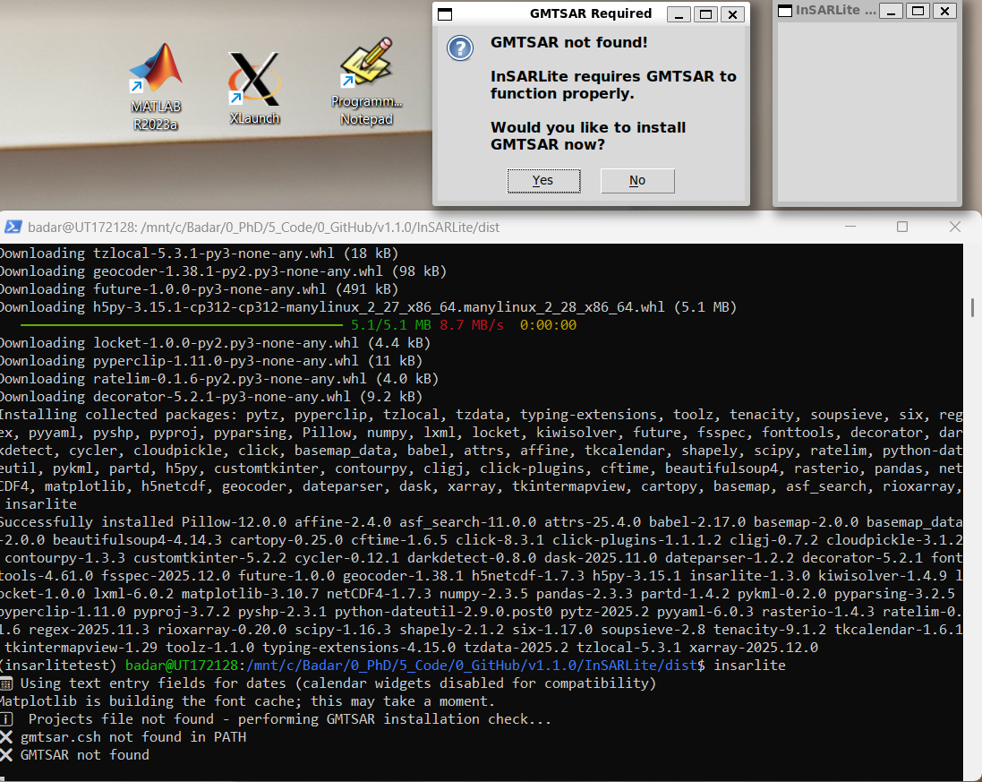
On first launch, InSARLite automatically checks for GMTSAR installation. If GMTSAR is not found, you’ll see this prompt offering automatic installation.
What’s shown: Main GUI is initially blank and compact. A prompt indicates GMTSAR is not found with the terminal output visible.
User Action: Click Yes to proceed with automatic installation.
Step 1.2: Installation Mode Selection
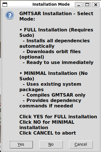
Choose between two installation modes:
Full Installation: Includes all GMTSAR components, dependencies, and full functionality
Minimal Installation: Basic functionality only (not recommended for this tutorial)
User Action: Select Full Installation for complete functionality.
Step 1.3: Optional Orbit Files
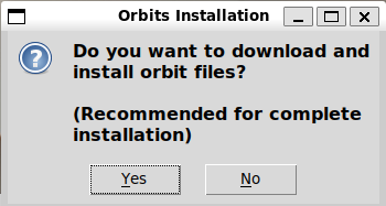
InSARLite can pre-download Sentinel-1 orbit files to save time later. This is optional as orbits can be downloaded on-demand.
User Action: Click No (orbits will be downloaded automatically when needed).
Step 1.4: Authentication
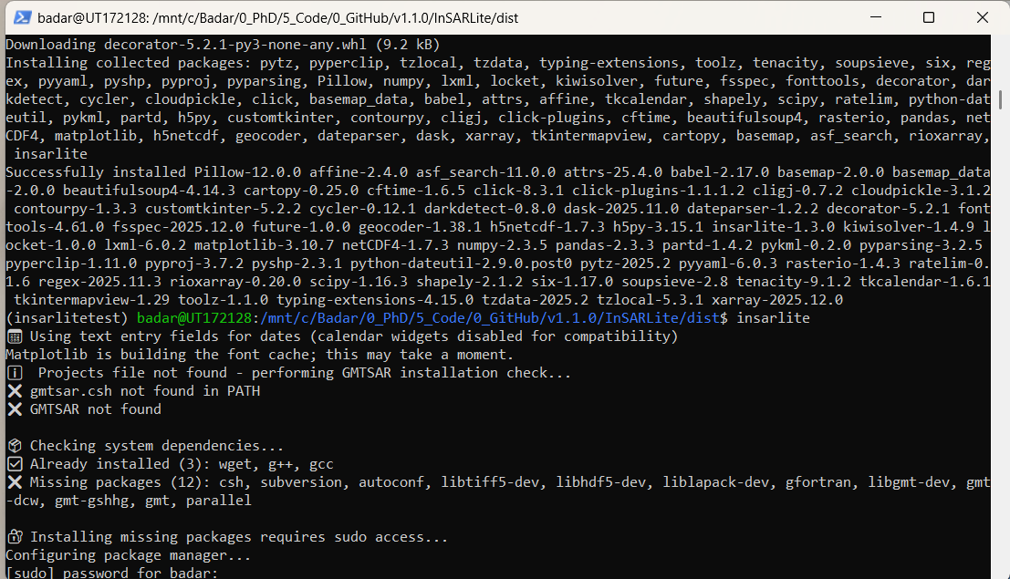
Full installation requires administrator privileges to install system dependencies.
User Action: Enter your sudo password when prompted.
Step 1.5: Installation Confirmation
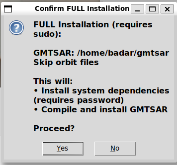
Review your selected options before proceeding:
Installation mode: Full
Orbit files: No
System modifications will be made
User Action: Click Yes to confirm and start installation.
Step 1.6: Installation Complete
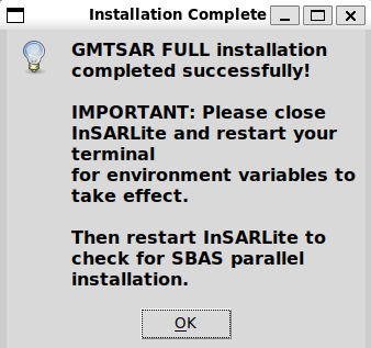
Installation successful! InSARLite recommends restarting to ensure environment variables are properly loaded.
User Action: Click OK.

InSARLite will now close to allow environment refresh.
User Action: Click OK.
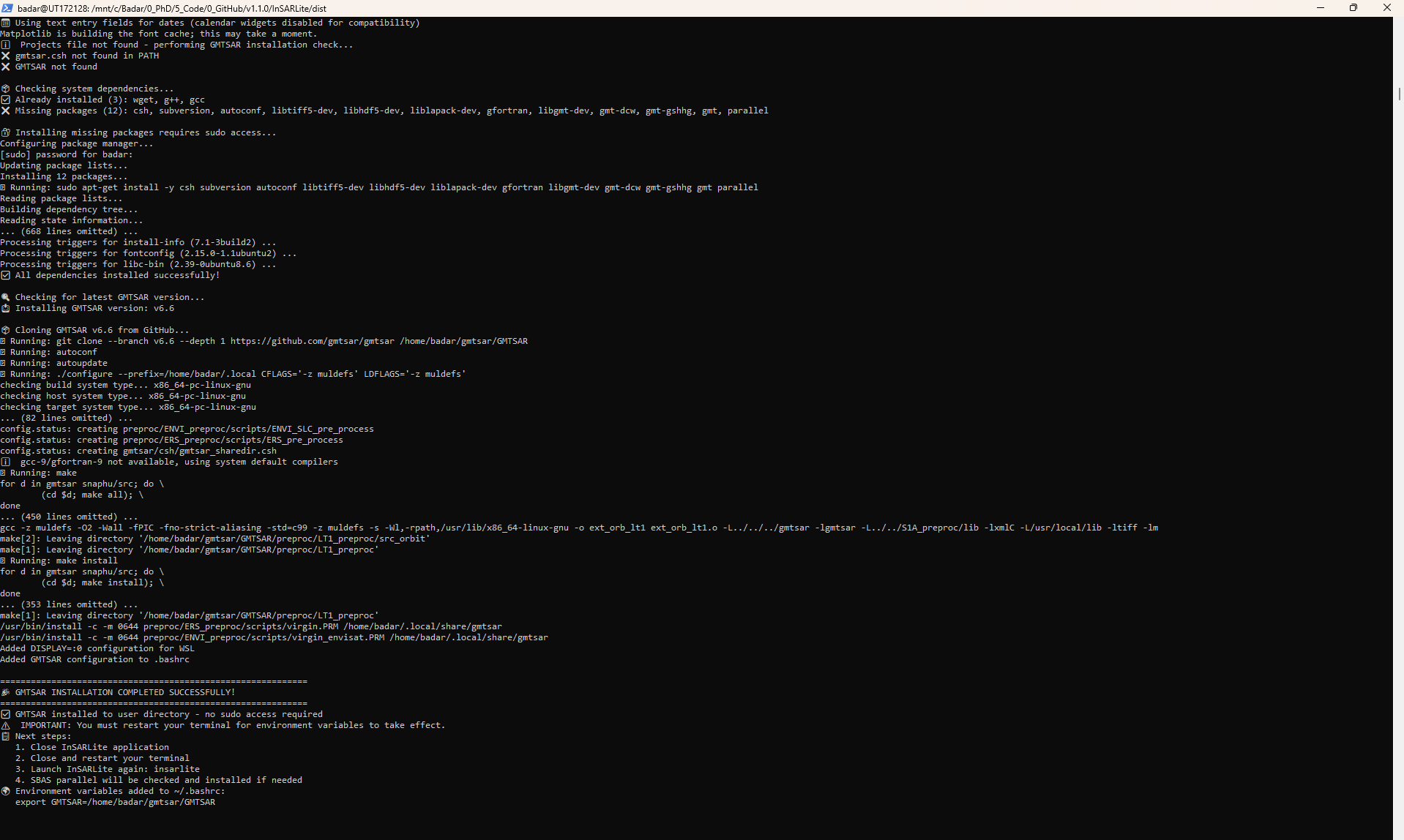
Terminal output confirms successful installation with all components properly configured.
Step 1.7: Verification
After restarting InSARLite, the main GUI will launch normally. You can verify GMTSAR installation by checking the terminal or running:
gmtsar.csh
If installation was successful, you’ll see GMTSAR version information.
Part 2: Project Configuration
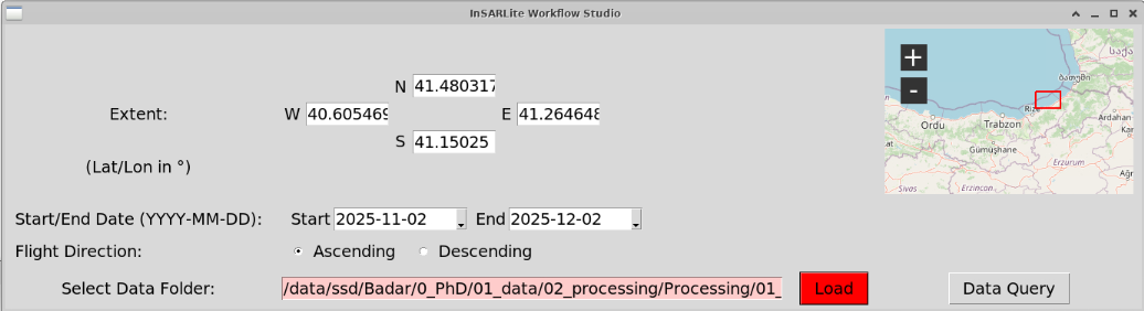
Step 2.1: Define Data Folder
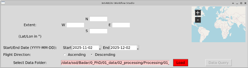
What’s shown: Main GUI with data folder defined as an empty directory. Red textbox background and red “Load” button indicate missing data.
User Action:
Click Browse to select an empty folder for your project
This folder will contain all downloaded and processed data
Step 2.2: Define Area of Interest (AOI)
What’s shown: Bounding box drawn on the interactive map, encompassing the Güngören landslide area. The map widget displays Sentinel-1 frame footprints and AOI extent.
User Action:
Use the map tools to draw a bounding box around your study area
The box should encompass the entire landslide region with some buffer
Click to set corners of the bounding box
Tip: Include surrounding stable areas for reference point selection later.
Step 2.3: Define Temporal Range
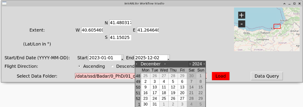
What’s shown: Calendar widget for selecting the end date of the analysis period.
User Action:
Set start date to capture sufficient pre-failure baseline
Set end date to include the failure event and some post-failure data
For this study: Start ~early 2023, End ~late 2024
Step 2.4: Query Available Data
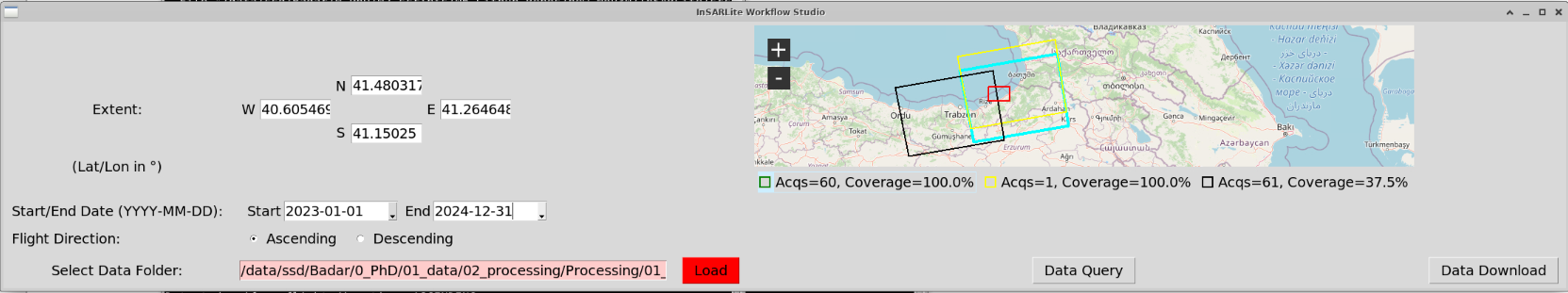
What’s shown: Query results showing available Sentinel-1 scenes that match the AOI and temporal criteria. Frame information and acquisition count are displayed.
User Action:
Review the query results
Check the number of available acquisitions (should show ~60 scenes)
Select the appropriate frame for download
Click Download Selected
Note: This query uses NASA’s Alaska Satellite Facility (ASF) API.
Step 2.5: Download Sentinel-1 Data
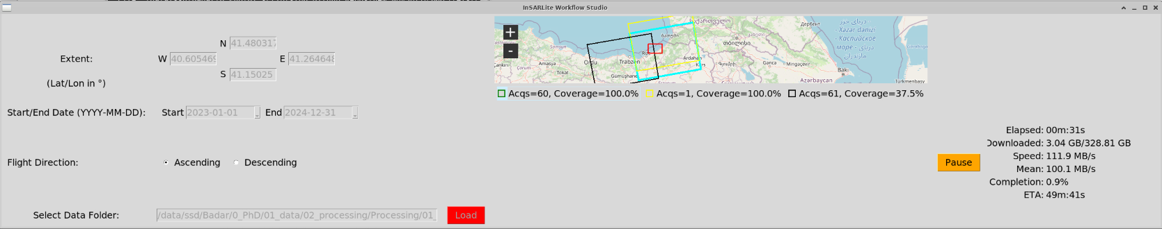
What’s shown: Active download progress with status indicators.
What happens: InSARLite downloads all selected Sentinel-1 .zip files from ASF to your data folder. Progress is shown in real-time.
Download size: 328.8 GB total (60 acquisitions: 23 files @ ~7.5 GB each, 37 files @ ~4.2 GB each)
What’s shown: GUI state when download completes. All .zip files are now in the data folder.
User Action: Click OK or proceed to extraction.
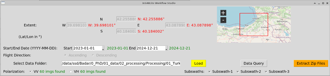
Step 2.6: Extract Sentinel-1 Data
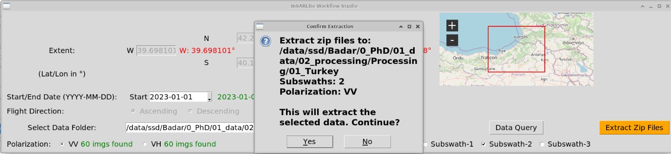
What’s shown: Extraction confirmation prompt with additional parameter options.
User Action:
Select subswath (IW2/F2 for this study)
Click Extract
Confirm extraction in the prompt
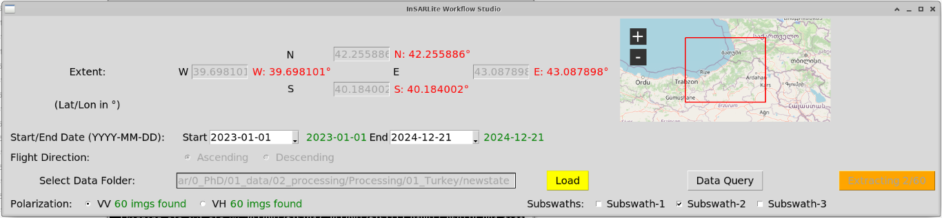
What’s shown: GUI state during extraction process.
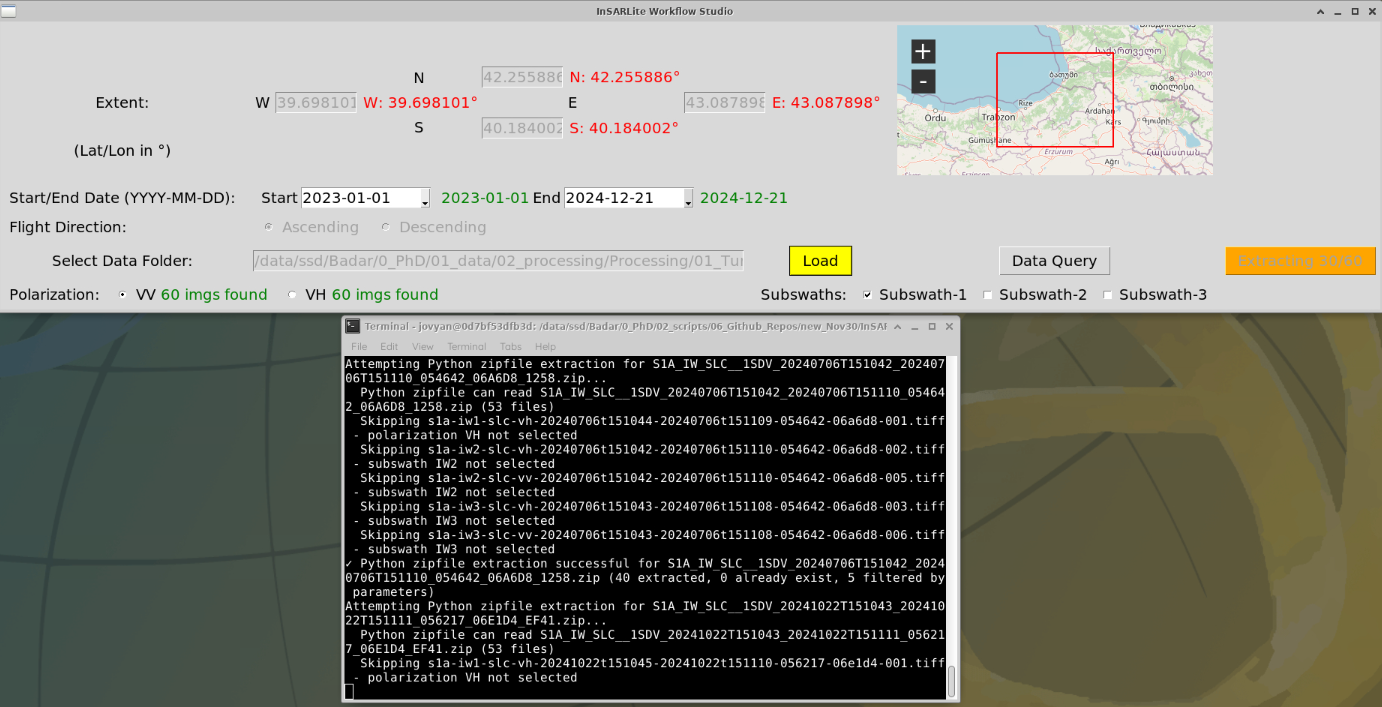
What’s shown: Detailed terminal output during extraction showing individual file processing.
What happens: InSARLite extracts .SAFE directories from .zip files, organizing data for GMTSAR processing.
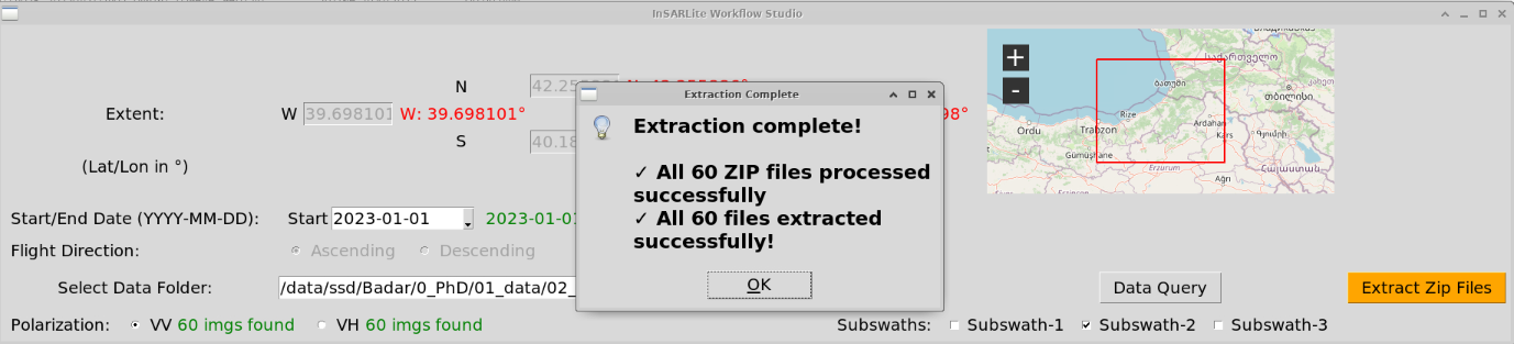
What’s shown: Extraction complete prompt with main GUI in background.
User Action: Click OK.
Step 2.7: Validate Data
What’s shown: GUI state showing valid SAFE directories confirmed. The data folder now contains properly extracted and organized Sentinel-1 data.
What happens: InSARLite automatically validates the extracted data structure, checking for:
Correct .SAFE directory format
Required XML metadata files
Measurement data files
Consistent subswath selection
Status indicators: Green confirmation shows all 60 acquisitions are valid.
Step 2.8: Download DEM
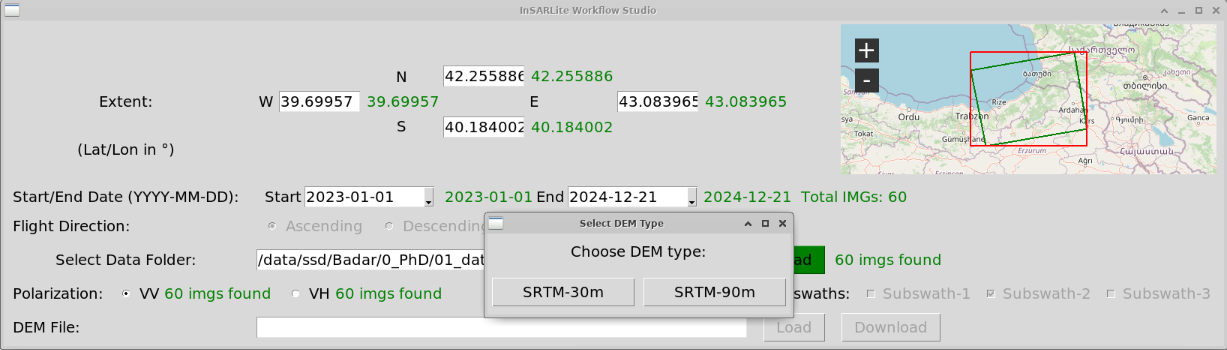
What’s shown: DEM download prompt with resolution options.
User Action:
Click Download DEM
Select resolution:
SRTM 1 arc-second (~30m): Higher resolution, recommended
SRTM 3 arc-second (~90m): Faster download, lower resolution
Recommendation: Use 30m DEM for detailed landslide analysis.
What happens: InSARLite automatically downloads SRTM DEM tiles covering your AOI and creates a merged, properly formatted DEM for GMTSAR.
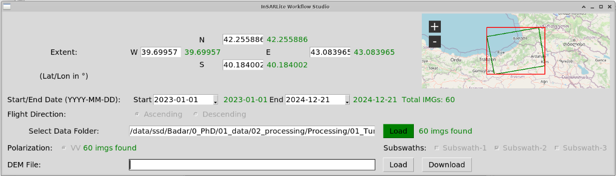
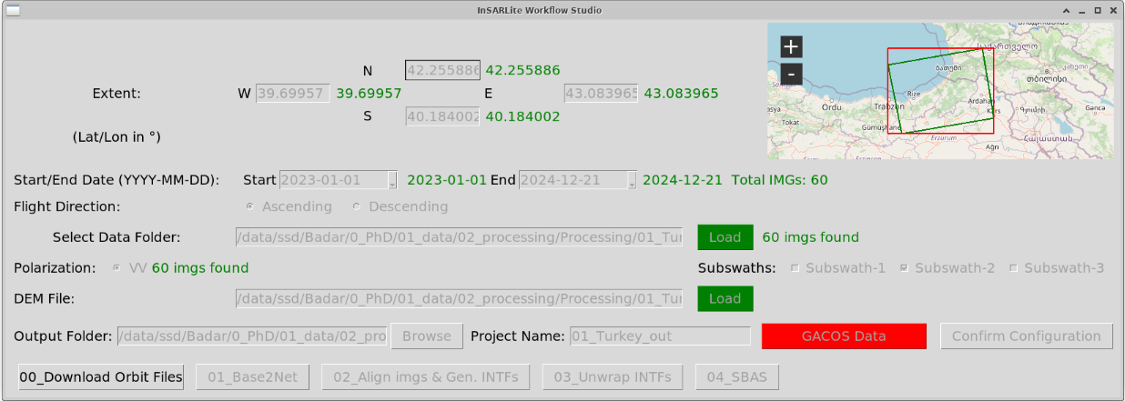
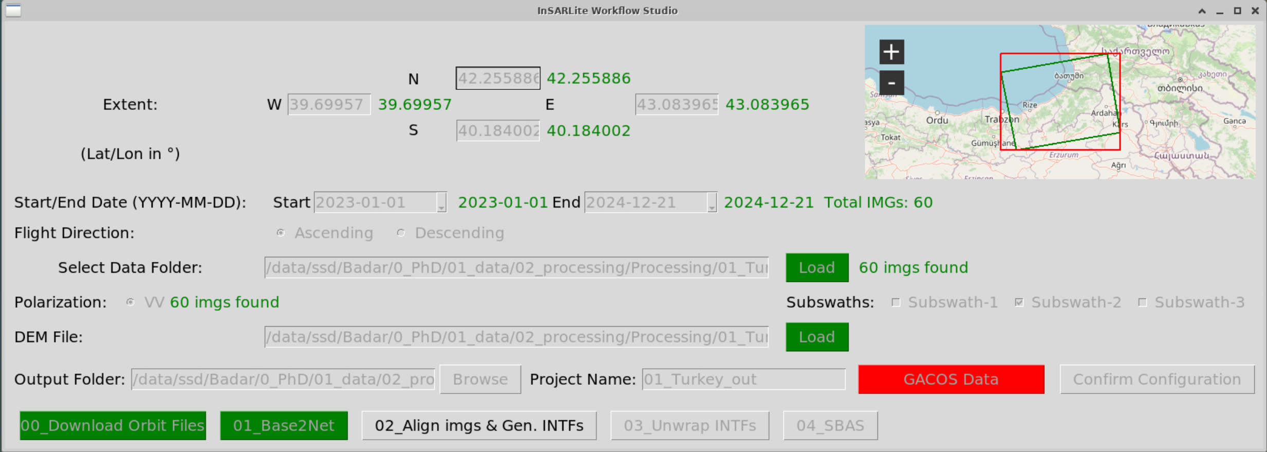
Step 2.9: Define Output Configuration
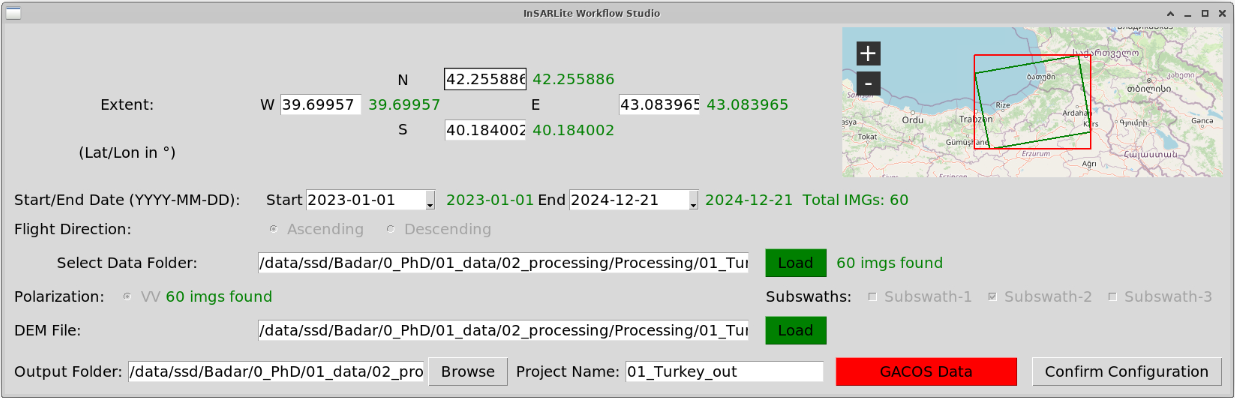
What’s shown: Main GUI state when all required parameters are defined but configuration not yet confirmed.
Parameters shown:
Data folder: Populated with valid data
AOI: Defined on map
Temporal range: Set
DEM: Downloaded
Output folder: To be specified
Project name: To be specified
User Action:
Specify output folder location
Enter a descriptive project name (e.g., “Gungoren_Landslide_2024”)
Do not click “Confirm Configuration” yet
What’s shown: Main GUI state after clicking “Confirm Configuration”.
What happens: InSARLite creates the complete directory structure for GMTSAR processing:
output_folder/asc/
├── data/          # Symlinks to original SAFE directories from data folder, orbit files
├── F2/             # IW2 subswath processing folder
│   ├── raw/        # Symlinks to IW2 files, baseline files, aligned images
│   ├── intf/       # Interferograms temporary directory
│   ├── intf_all/   # Interferograms (moved here after creation)
│   └── topo/       # DEM and topographic products
├── SBAS/           # Time series results
├── topo/           # DEM and topographic products
└── reframed/       # Location of pin.ll file with coordinates of two pins covering S1 frame
User Action: Click Confirm Configuration.
Status: Project is now fully configured and ready for processing!
Part 3: Baseline Network Design (Step 1)
Step 3.1: Download Precise Orbit Files
What’s shown: GUI state after Step 00 (orbit download) completion.
User Action: Click 00_Download Precise Orbits.
What happens: InSARLite automatically downloads precise orbit ephemerides (POE) files from ESA for all 60 acquisitions. These files provide accurate satellite positions essential for interferometric processing.
Processing time: 2-5 minutes (depends on internet speed).
Step 3.2: Open Baseline Calculator (Base2Net)
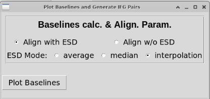
What’s shown: “Baseline calc. & Align. Param.” controls in default state.
Parameters visible:
ESD (Enhanced Spectral Diversity) options
Alignment parameters
Default selections loaded
User Action: Review default parameters, then click Calculate Baselines.
Step 3.3: Plot Baselines
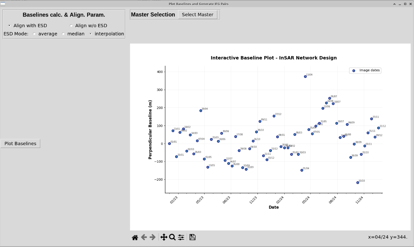
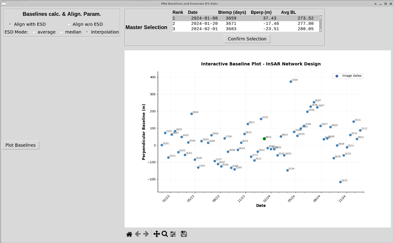
What’s shown: Base2Net interface with baselines plotted on the temporal-perpendicular baseline graph.
Graph shows: All 60 acquisitions plotted with:
X-axis: Date (mm/yy format), with each point labeled as dd/mm and positioned by temporal baseline
Y-axis: Perpendicular baseline (meters)
User Action: Click Select Master to proceed with master image selection.
Interpretation: The baseline plot shows the spatial-temporal distribution of acquisitions. Widely scattered acquisitions require careful master selection to minimize decorrelation.
Step 3.4: Calculate Master Table
Warning:
The procedure below is intended as guidance for master-image selection and does not guarantee the optimal master for every dataset. You may choose any acquisition as the master; the metrics computed here are provided only to support an informed decision.
What’s shown: Master table calculated and displayed, ranking all acquisitions by suitability as master image.
What’s calculated: Network centrality for each acquisition using:
where:
\(C_i\) = centrality score for acquisition \(i\)
\(B_{\perp,ij}\) = perpendicular baseline between acquisitions \(i\) and \(j\)
\(T_{ij}\) = temporal baseline between acquisitions \(i\) and \(j\)
\(B_{\text{crit}}\) = critical perpendicular baseline (typically 150-300m)
\(T_{\text{crit}}\) = critical temporal baseline (typically 48-96 days)
Table columns:
Rank: Sorted by ascending average baseline (lowest = best)
Date: Acquisition date
Btemp (days): Temporal baseline value relative to first acquisition
Bperp (m): Mean perpendicular baseline relative to other acquisitions
Avg BL: Average baseline metric (corresponds to centrality score)
Best master: Acquisition with lowest average baseline (highest centrality score = most connections to other scenes).
Step 3.5: Select Master Image
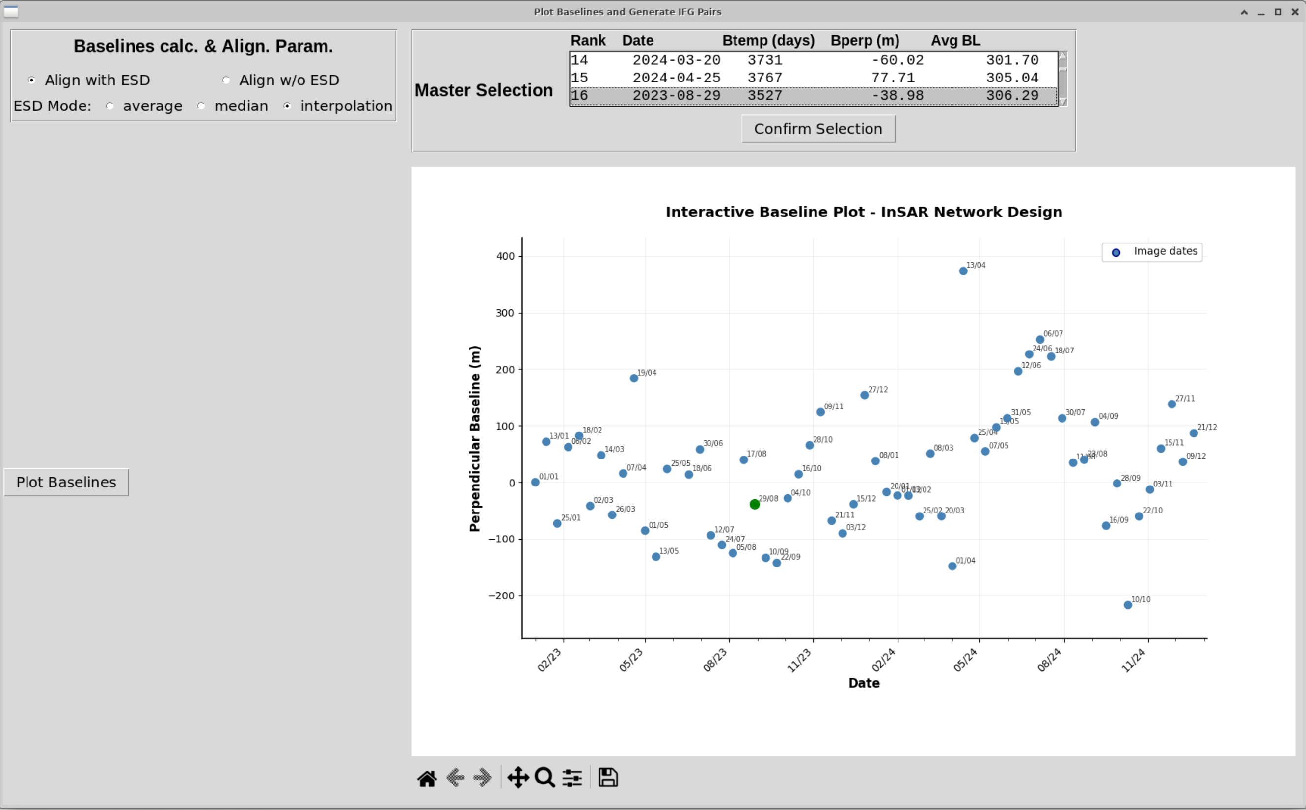
What’s shown: Entry ranked 16 selected as master image.
Master Details:
Date: August 29, 2023
Rank: 16
Rationale for Rank 16 Selection:
This tutorial intentionally selects rank 16 (rather than rank 1) to emphasize that master-image selection is entirely up to the user:
SBAS vs PSI Master Selection:
PSI (Persistent Scatterer): Requires optimal master with lowest average baseline because ALL interferograms reference this single master. Master quality critically affects entire dataset coherence.
SBAS (Small Baseline Subset): Uses multi-master configuration where interferograms are formed between temporally adjacent acquisitions. The “master” only serves as an alignment reference for image coregistration, not as a single interferometric reference.
In SBAS processing, master selection is far less critical than in PSI because:
Each interferogram uses its own optimal pair (small temporal/spatial baselines)
Time series inversion handles multiple reference configurations
Coherence is maintained through small baseline subsets, not single-master connectivity
User Action:
Review the ranked list
Select rank 16 (as demonstrated) or rank 1 (optimal by metric)
Click Confirm Selection
Step 3.6: Define Baseline Constraints
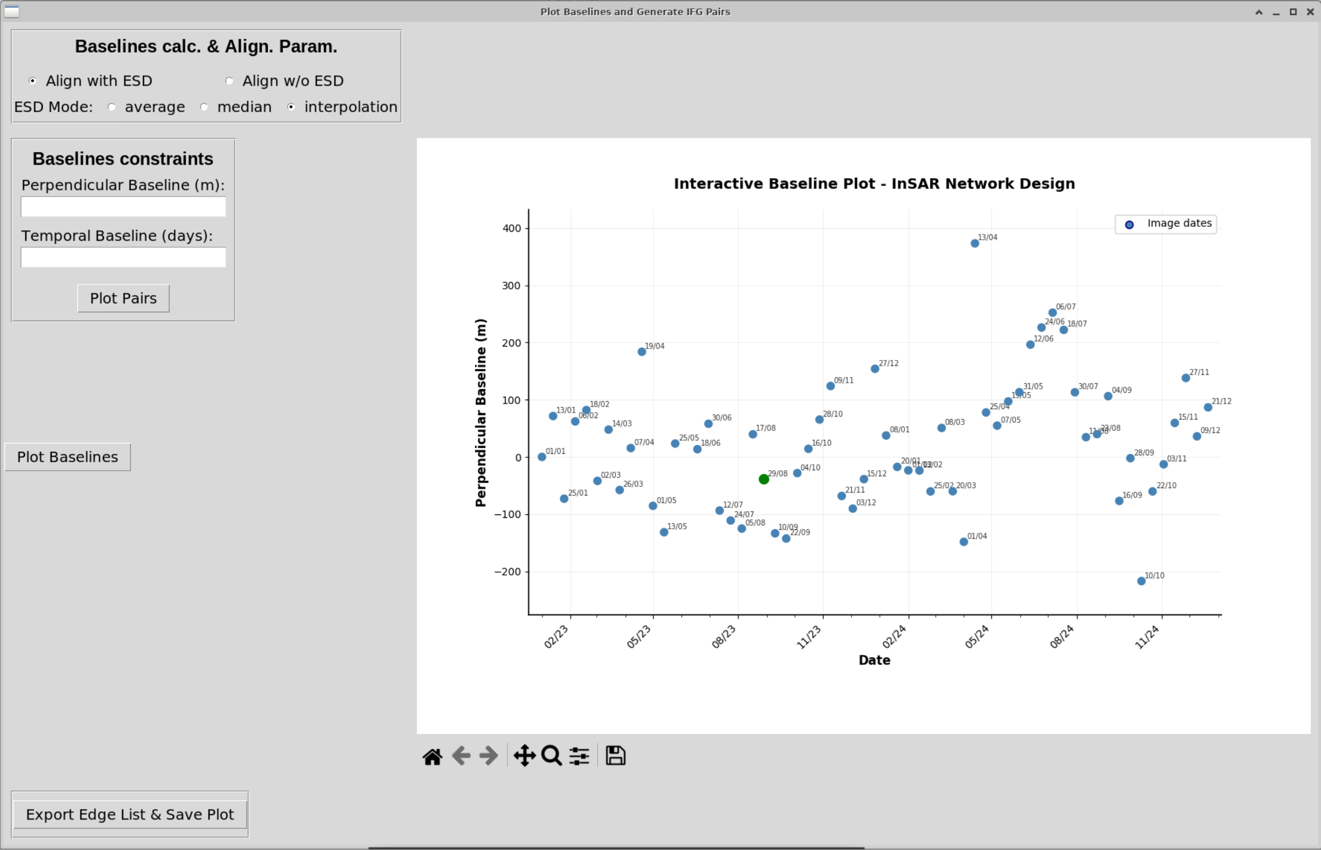
What’s shown: Baseline constraints controls now visible after master selection.
User Action: Define thresholds for interferogram pair selection:
Perpendicular baseline threshold: Maximum spatial baseline (in meters)
Temporal baseline threshold: Maximum time separation (in days)
Preparation: Ready to define constraints and generate interferometric pairs.
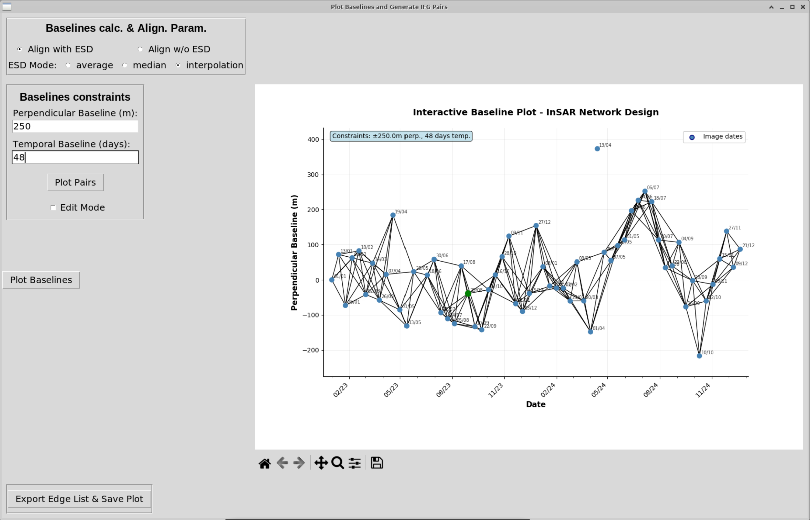
What’s shown: Constraints defined and interferometric pairs plotted.
Constraints used:
Perpendicular baseline: 250 meters (maximum)
Temporal baseline: 48 days (maximum)
Graph shows: Network connections between master and slave acquisitions that meet the criteria. Lines represent interferometric pairs to be generated.
User Action: Click Plot Pairs to visualize the network.
Network characteristics:
Small Baseline Subset (SBAS) approach
Ensures sufficient temporal sampling
Minimizes decorrelation effects
Creates redundant network for robust inversion
Step 3.7: Export Network Configuration
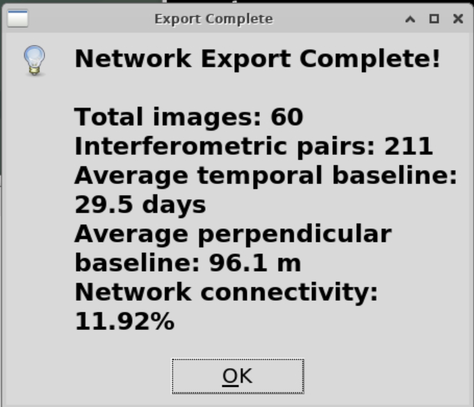
What’s shown: Export complete prompt.
What’s exported:
baseline_table.dat: Baseline information for all pairsintf.in: List of interferometric pairs to generateNetwork configuration plots (PNG/PDF)
User Action: Click Export.
Files created: These files are used by GMTSAR in subsequent processing steps.
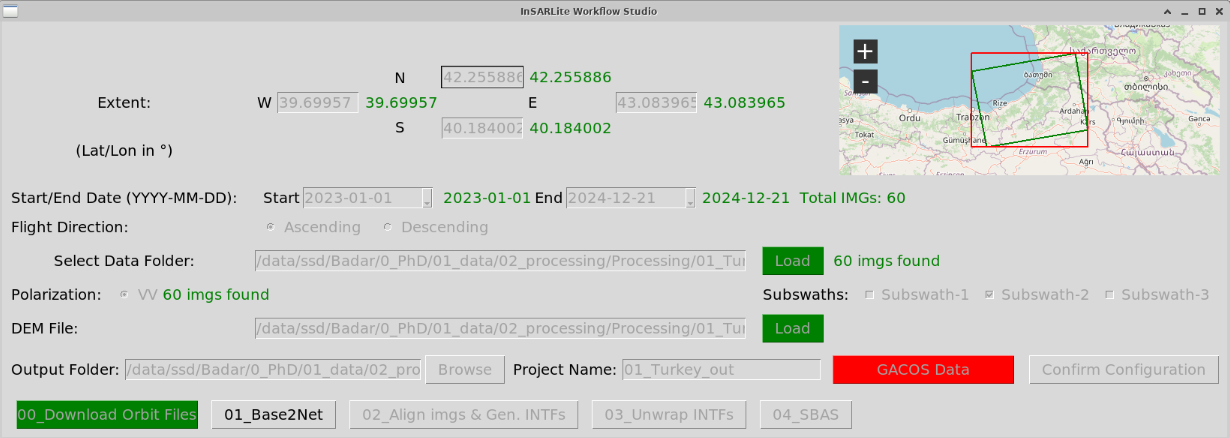
What’s shown: Back to main GUI after Base2Net process completion.
Status: Step 1 (Baseline Network Design) is complete. The GUI now shows:
Green/completed status for Step 1
Step 2 (Align & Generate IFGs) now active and ready
User Action: Click OK on the completion prompt.
Summary: You’ve successfully:
Downloaded precise orbits
Calculated baselines for all acquisitions
Selected an optimal master image (Aug 29, 2023)
Defined network constraints (250m, 48 days)
Generated interferometric pair list
Exported configuration for GMTSAR
Part 4: Interferogram Generation (Step 2)
Step 4.1: Configure IFG Parameters
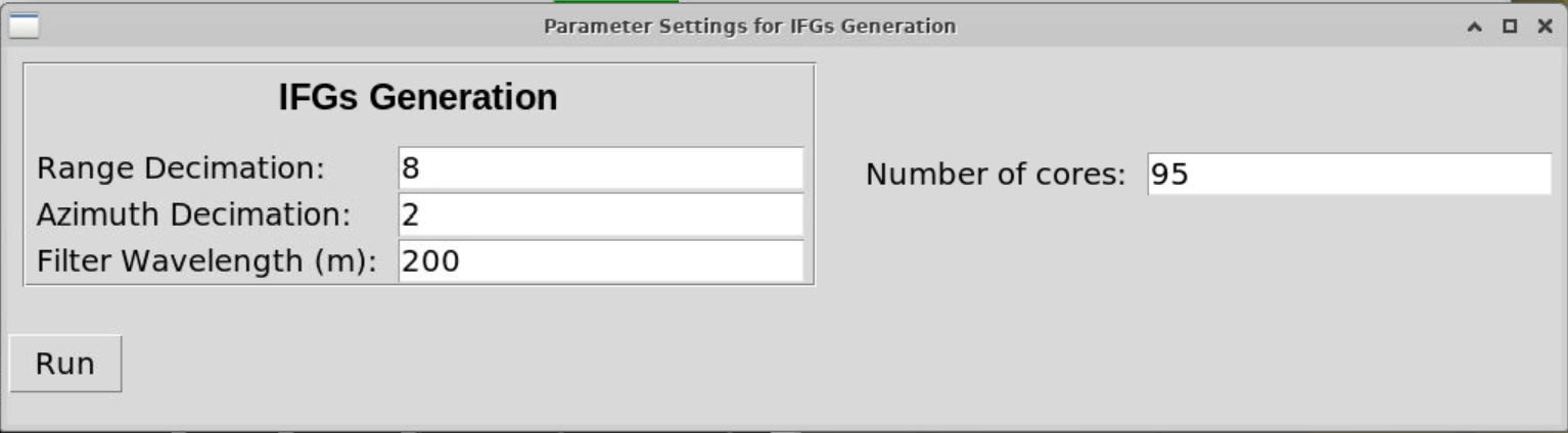
What’s shown: Interferogram generation GUI with default parameters.
Key parameters:
Range decimation: Reduces resolution in range direction (trade-off: speed vs. detail)
Azimuth decimation: Reduces resolution in azimuth direction
Filter wavelength: Gaussian filter for noise reduction (in meters)
Processing cores: Number of parallel threads (use all available)
Default values: Generally optimal for most applications.
User Action:
Review parameters (defaults are good for this tutorial)
Adjust cores to match your CPU (e.g., 8 cores)
Click Run
Recommendation: For landslide analysis, use minimal decimation to preserve detail.
Step 4.2: Confirm Execution
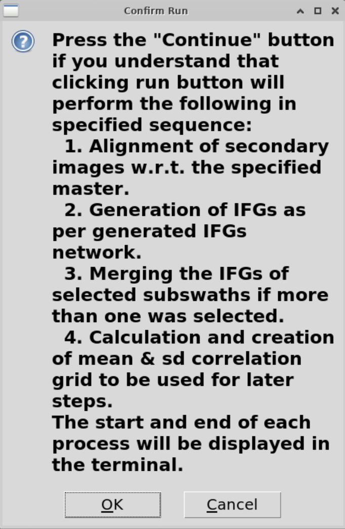
What’s shown: Confirmation prompt reviewing settings before execution.
What will happen:
Align all SAR images to master geometry
Generate interferograms for all pairs in
intf.inCalculate mean correlation (coherence)
Prepare data for unwrapping
Processing time estimate: 2-3 hours (depends on number of pairs and CPU cores).
User Action: Click OK to start processing.
Step 4.3: Monitor Processing Progress
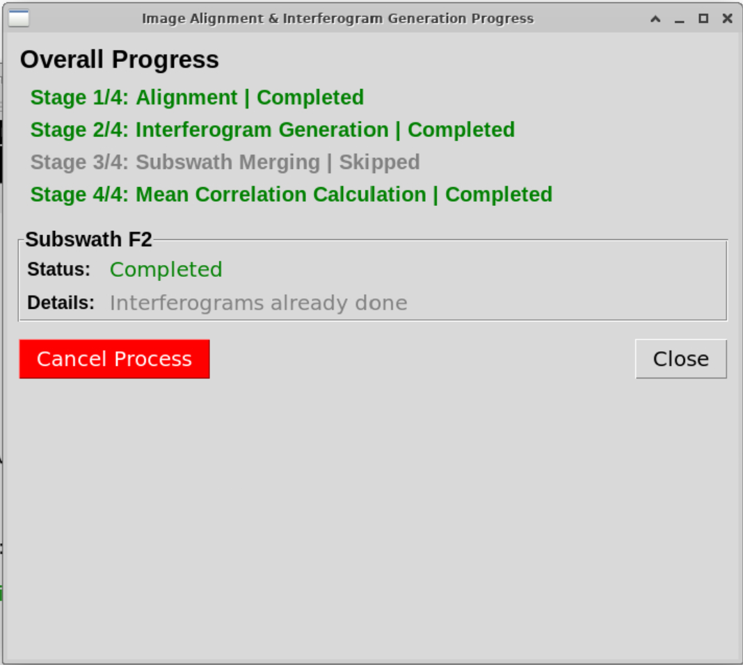
What’s shown: Progress GUI showing processing stages 1-4.
Processing stages:
Stage 1: Image alignment to master
Co-registers all acquisitions to master geometry
Creates aligned SLC images
Stage 2: Interferogram generation
Computes complex interferograms for all pairs
Applies topographic phase removal using DEM
Generates wrapped phase products
Stage 3: Subswath merging
Skipped (only F2/IW2 being processed)
Would merge IW1, IW2, IW3 if multiple subswaths selected
Stage 4: Mean correlation calculation
Computes average coherence across all interferograms
Creates
corr_stack.grdandstd.grdUsed later for mask definition
Real-time updates: Terminal output shows detailed progress for each pair.
User Action: Monitor progress, close window when complete.
What’s created:
F2/
├── raw/              # Aligned SAR images
│   └── *.SLC         # Single Look Complex images (all aligned to master)
├── intf_all/         # All interferograms
│   └── 2023XXX_2024XXX/
│       ├── phasefilt.grd     # Filtered wrapped phase
│       ├── corr.grd           # Correlation grid file
├── corr_stack.grd      # Mean correlation (to aid in masking and reference point selection)
└── std.grd      # Correlation std deviation
Processing complete: Step 2 finished. Ready for unwrapping!
Part 5: Phase Unwrapping (Step 3)
Phase unwrapping is a critical and computationally intensive process divided into 2 phases in InSARLite consisting cumulatively of 4 distinct steps:
Mask definition (optional)
Unwrapping process (of all wrapped interferograms)
Reference point selection
Unwrapping completion
Phase 1: Mask Definition
Step 5.1.1: Open Unwrap Interface
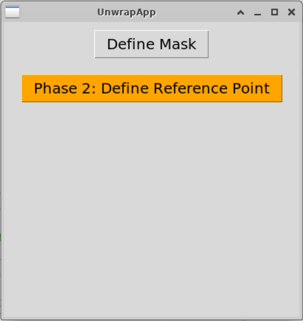
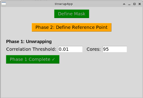
What’s shown: Default UnwrapApp state showing two main buttons:
Define Mask: Create/modify unwrapping mask
Phase 2: Currently inactive (will activate after Phase 1)
User Action: Click Define Mask to define/skip the unwrapping mask.
Why mask?: Unwrapping is only reliable in coherent areas. A mask excludes low-coherence pixels to prevent error propagation and dramatically reduce the computational requirements.
Step 5.1.2: Handle Existing Mask
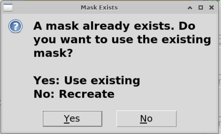
What’s shown: In case of an existing mask, users are asked if they want to use the existing one or create a new one.
User Action: Click Yes to recreate the mask fresh.
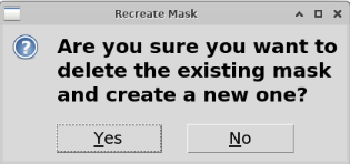
What’s shown: Confirmation to delete existing mask and create new one.
User Action: Click Yes to delete and recreate.
Step 5.1.3: Define Correlation Threshold
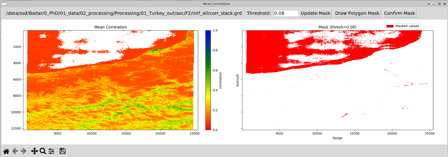
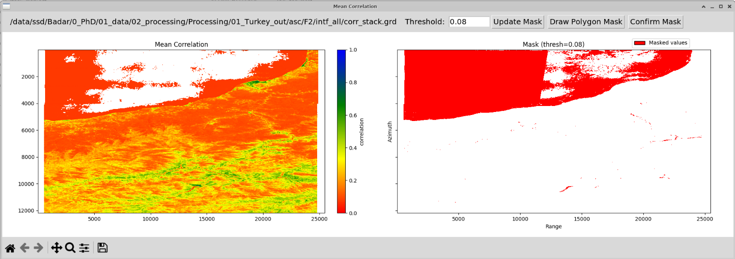
What’s shown: Mean correlation GUI for threshold-based masking.
Parameters:
Threshold: 0.08 (correlation values below this are masked out)
Display shows mean correlation map
User Action:
Set threshold to 0.08. The idea is to exclude ocean pixels.
Click Update Mask
Visualize the mask on the correlation map
Interpretation:
Red/low values: Low coherence (water, vegetation, steep slopes)
Green/high values: High coherence (bare ground, stable areas)
Threshold of 0.08 excludes very low coherence while retaining landslide area
Step 5.1.4: Add Polygon Mask
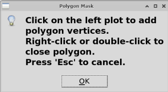
What’s shown: Polygon mask prompt offering option to add manual delineation.
Why polygon?: Sometimes you want to:
Exclude problematic regions manually
Refine threshold-based mask where any specific mean correlation value alone may exclude valid (land) pixels or include a lot of ocean pixels for unwrapping.
User Action: Click Polygon to draw manual mask.
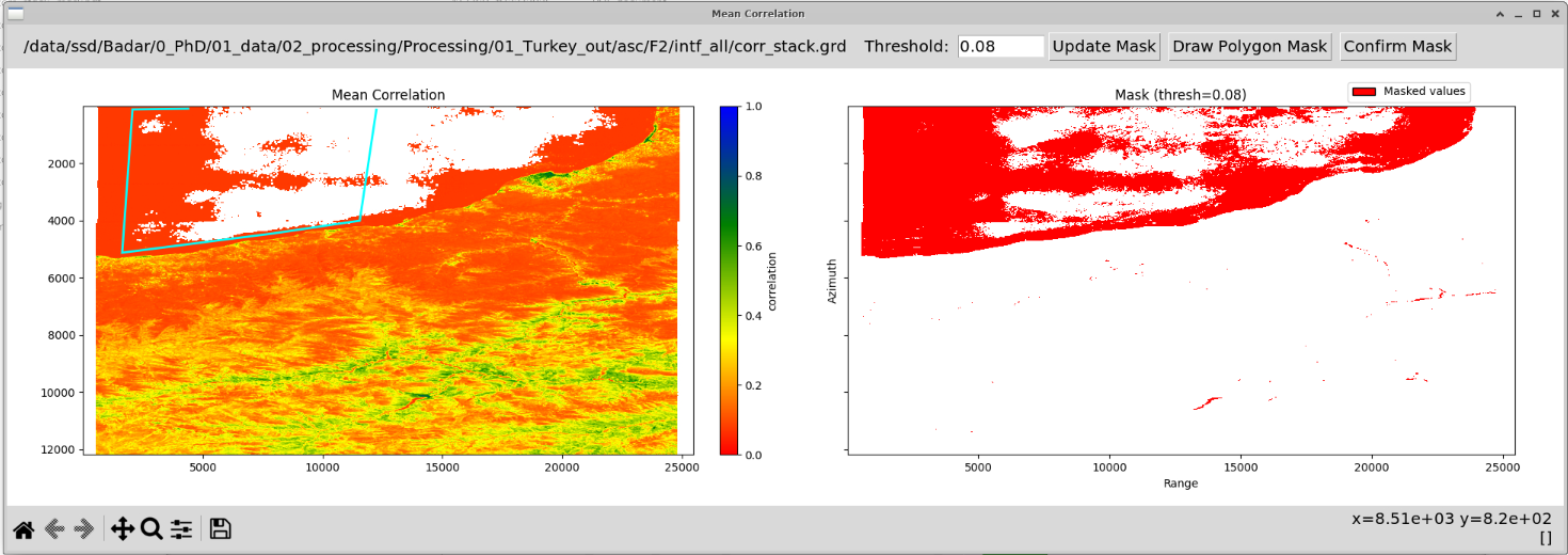
What’s shown: One polygon drawn on the correlation map (cyan outline). Multiple polygons can be drawn and a composite mask can be created. This case study uses two polygons to mask out oceans along with the mean correlation threshold value of 0.08 for masking. Delineation of only the first polygon is shown here.
User Action:
Click to place vertices around your area of interest
Right-click to complete the polygon
Polygon encloses the landslide area
Tip: Include some stable area outside the landslide for reference.
What’s shown: Polygon mask confirmation prompt.
User Action: Click Yes to confirm the polygon.
Step 5.1.5: Visualize Composite Mask
What’s shown: Composite mask displayed combining:
Correlation threshold (0.08)
Polygon mask (manual delineation)
Mask logic: Only pixels that satisfy BOTH conditions are included:
Correlation > 0.08 AND
Inside polygon
Result: A refined mask focusing on coherent pixels within the landslide area.
Step 5.1.6: Export Mask
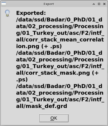
What’s shown: Export prompt.
What’s exported: Mask file applied to all interferograms for unwrapping.
User Action: Click Export.
File created: mask_def.grd used in unwrapping.
Phase 2: First Unwrapping
Step 5.2.1: Run Phase 1 Unwrapping
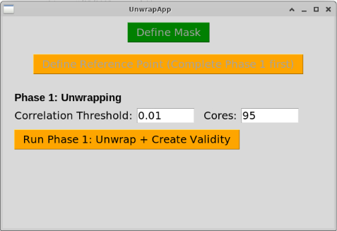
What’s shown: Back to UnwrapApp after defining mask.
Status: Mask is defined and exported. Ready for first unwrapping pass.
User Action: Click Run Phase 1:…
What happens: GMTSAR’s SNAPHU unwrapper runs on all interferograms with the defined mask.
Step 5.2.2: Unwrapping Completion
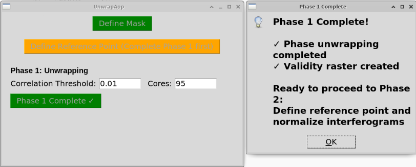
What’s shown: Phase 1 completed with parameters:
Threshold: 0.01 (default SNAPHU threshold)
Number of cores: 95 (A default value is auto-filled depending on the CPU, as number of threads available - 1)
Processing: SNAPHU uses statistical-cost, network-flow algorithm for phase unwrapping.
User Action: Click OK.
What’s created: Unwrapped phase files for all interferograms.
What’s shown: Phase 2 controls now active after Phase 1 completion.
Status: Interferograms are unwrapped but not yet normalized to a common reference point.
User Action: Proceed to reference point selection.
Phase 3: Reference Point Selection
Step 5.3.1: Check for Existing Reference
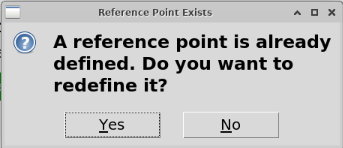
What’s shown: When applicable, this prompt allows the user to choose an existing reference point or to select a new one instead of the existing one.
User Action: Click Yes to redefine reference point.
Why redefine?: You may want to change reference point for better stability or scientific reasons.
Step 5.3.2: Open Enhanced Reference Point Selection
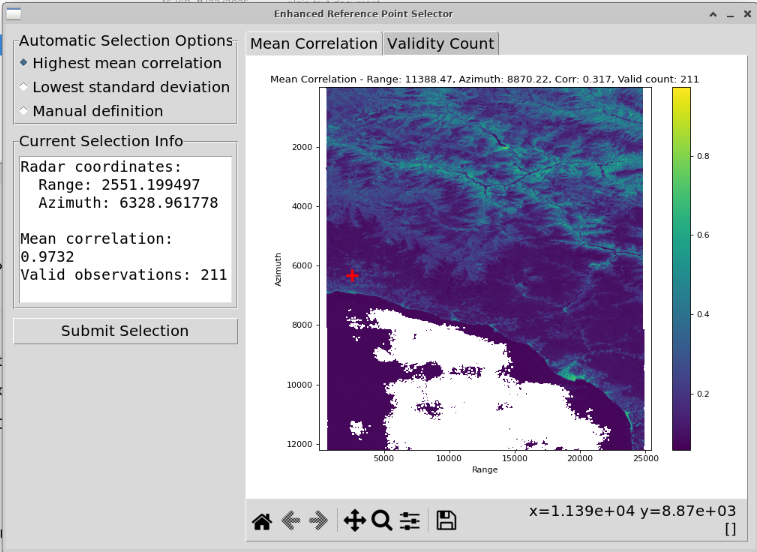
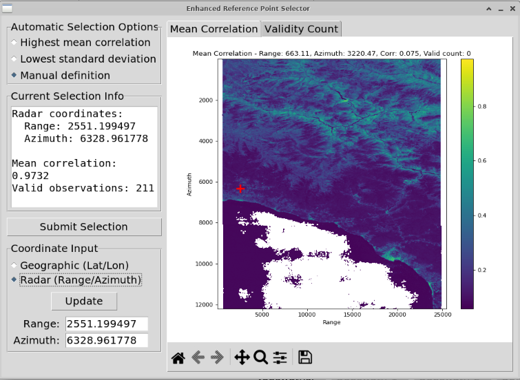
What’s shown: Enhanced reference point selection interface with multiple selection methods.
Default selection: “Highest mean corr” is automatically selected, showing the location with the highest average correlation.
Why this matters: The reference point should be:
Stable (no deformation)
Highly coherent (reliable phase measurements)
Outside the deforming area
Display: Mean correlation map with cursor showing current reference point location.
Step 5.3.3: Explore Selection Options
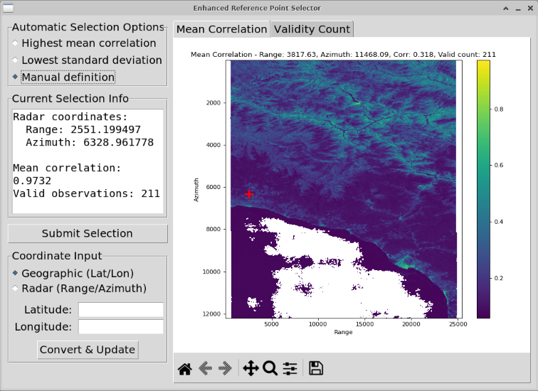
What’s shown: Manual definition controls visible.
Selection methods available:
Automated:
Highest mean correlation (default selection)
Lowest std deviation of correlation
Manual:
Click on mean correlation map
Click on validity count map
Enter coordinates directly (geographic or radar)
What’s shown: Radar coordinate option selected for manual entry.
Coordinate systems:
Radar: Range and azimuth pixel coordinates
Geographic: Latitude and longitude
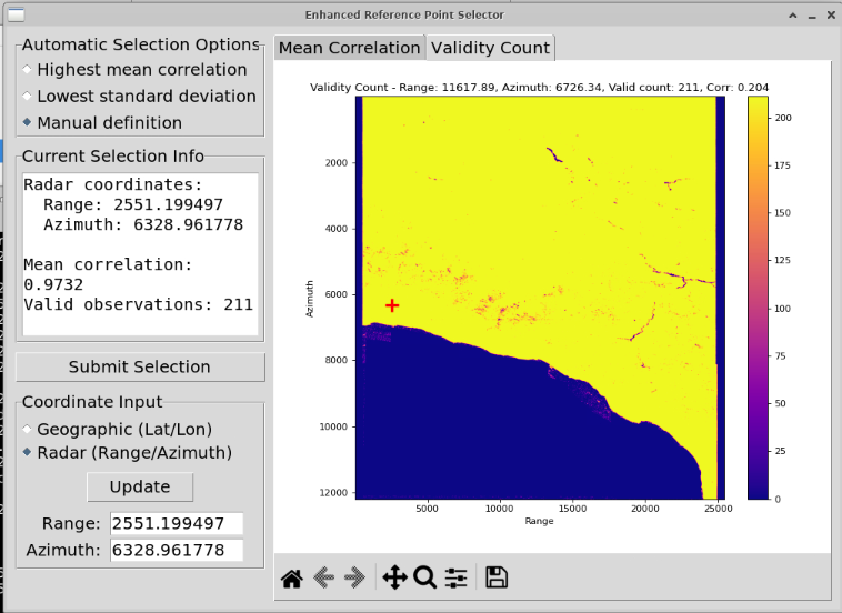
What’s shown: Validity Count tab active with radar coordinates.
Validity count: Number of interferograms with valid unwrapped phase at each pixel.
Use case: Select reference point with maximum validity (appears in most interferograms).
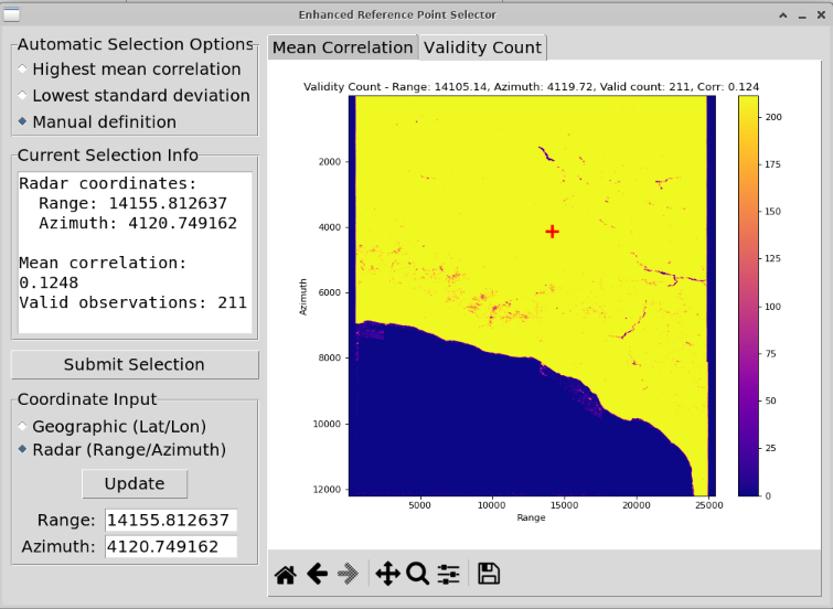
What’s shown: Different location clicked on validity map, values updated.
Interactive: Click anywhere on the map to evaluate potential reference points.
Evaluation criteria:
High mean correlation
Low correlation std deviation
High validity count
Located in stable area (away from landslide)
Step 5.3.4: Confirm Reference Point
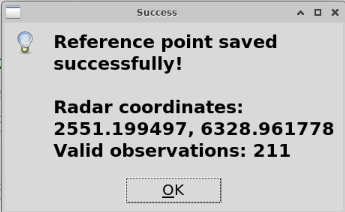
What’s shown: Success prompt after selecting reference point.
Reference selected: Highest mean correlation location (automated selection).
Coordinates:
Range: 2551.199497
Azimuth: 6328.961778
User Action: Click OK to apply reference point.
What happens: All interferograms are normalized to this reference point, setting it as zero deformation.
Phase 4: Unwrapping Completion
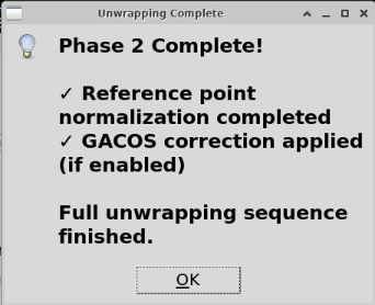
What’s shown: Unwrapping complete prompt.
Status: All interferograms are:
✅ Unwrapped
✅ Masked
✅ Normalized to reference point
✅ Ready for SBAS inversion
User Action: Click OK.
Files created:
F2/intf_all/2023XXX_2024XXX/
├── unwrap.grd           # Unwrapped phase
├── unwrap_pin.grd      # Normalized Unwrapped phase
Summary: Step 3 complete! You’ve successfully:
Created a composite mask (threshold + polygon)
Unwrapped all interferograms
Selected optimal reference point
Normalized all phases to common reference
Part 6: SBAS Inversion and Visualization (Step 4)
Step 6.1: Configure SBAS Parameters
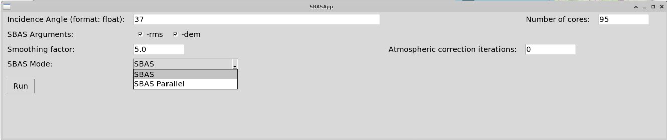
What’s shown: SBASApp interface with SBAS Mode dropdown clicked.
SBAS modes:
SBAS (standard): Sequential processing
SBAS parallel: Multi-core parallel processing (faster)
User Action: Select SBAS parallel for faster processing.
Other parameters:
Smoothing: Spatial smoothing factor (0.0 = no smoothing)
Atmospheric iterations: Number of iterations for atmospheric correction (default: 3)
Wavelength: Radar wavelength (calculated from metadata of all input images automatically. For more details, please refer to GMTSAR documentation for the exact equation and theory.)
Step 6.2: Confirm Existing Displacement Files
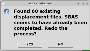
What’s shown: When valid, a prompt asks the user whether to rerun the process or skip it.
What this means: All interferograms have been successfully unwrapped and are ready for inversion.
User Action: Click OK to proceed.
Background: SBAS creates disp_*.grd files (unwrapped phase converted to line-of-sight displacement) for each input image epoch as well as a vel.grd file showing the overall velocity value of each pixel.
Step 6.3: Execute SBAS Inversion
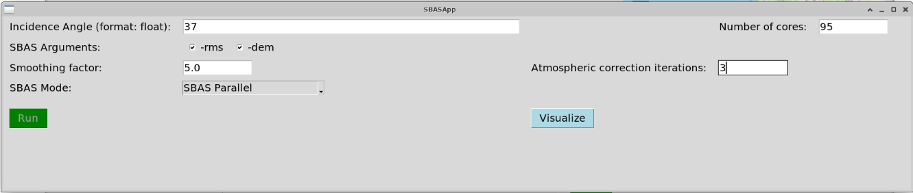
What’s shown: SBAS completed successfully with parameters:
Mode: SBAS parallel
Atmospheric iterations: 3
Smoothing: 0.0 (default)
What happened: Small Baseline Subset inversion solved for displacement time series at each pixel.
SBAS method: Solves the following system for each pixel:
where:
\(\mathbf{G}\) = design matrix (network geometry)
\(\mathbf{m}\) = displacement time series (unknowns)
\(\mathbf{d}\) = observed interferometric phase (data)
Solution: Least-squares inversion with optional smoothing:
where \(\alpha\) = smoothing factor, \(\mathbf{L}\) = Laplacian operator.
Status: “Visualize” button now active (cyan).
User Action: Click Visualize to launch interactive visualization.
Files created:
SBAS/
├── disp_YYYYMMDD.grd    # Displacement at each epoch
├── vel.grd              # Mean velocity (mm/yr)
├── rms.grd              # RMS of fit (optional)
└── dem_err.grd        # DEM error estimate (optional)
Step 6.4: Launch Surface Deformation Visualizer
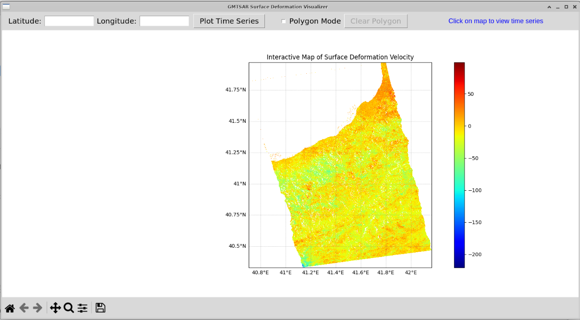
What’s shown: Default visualization showing mean LOS velocity map.
Features:
Interactive map: Pan, zoom, click pixels
Color scale: Velocity in mm/yr
Deformation pattern: Clear signal in landslide area
Basemap: Coordinate grid and frame extent
Automatic processing on launch:
✅ Reproject velocity to geographic coordinates
✅ Create velocity KML for Google Earth
✅ Reproject time series to geographic coordinates
✅ Load all time series into memory
✅ Generate interactive velocity map
Interactive capabilities:
Click any pixel → view time series
Zoom and pan
Export plots (PNG/EPS/PDF/SVG)
Export data (CSV)
Polygon mode for multi-pixel analysis
Interpretation:
Red: Movement toward satellite (uplift or eastward)
Blue: Movement away from satellite (subsidence or westward)
Landslide area: Strong blue signal indicating movement away from satellite (downslope motion with LOS component)
Step 6.5: Polygon Mode Analysis
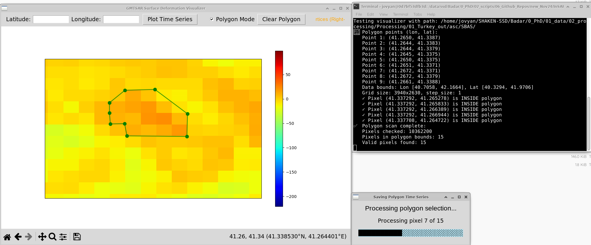
What’s shown: Polygon Mode active with:
Map zoomed to landslide area
9-vertex polygon drawn around deforming area
Terminal messages showing processing progress
Progress prompt: “Processing pixel 7 of 15”
User Action:
Click Polygon Mode button
Zoom/pan to area of interest
Click to place vertices (9 vertices in this case)
Right-click to complete polygon
Confirm polygon
Wait for processing (15 pixels extracted)
What happens: InSARLite:
Extracts all pixels within polygon
Plots individual time series for each pixel
Saves plots in multiple formats
Saves data in CSV format
Generates location maps
Processing time: ~30 seconds for 15 pixels.
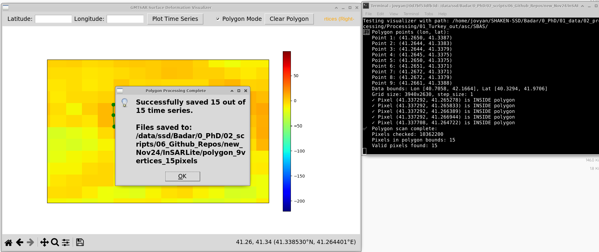
What’s shown: Polygon processing complete with:
Completion prompt displayed
Terminal output showing successful completion
All files saved notification
User Action: Click OK.
Files generated (for each pixel in polygon):
SBAS/time_series/polygon_9vertices_15pixels/
├── timeseries_N41p3373_E41p2658.png  # Time series plot
├── timeseries_N41p3373_E41p2658.eps  # Vector format
├── timeseries_N41p3373_E41p2658.pdf  # Vector format
├── timeseries_N41p3373_E41p2658.svg  # Vector format
├── timeseries_N41p3373_E41p2658.csv  # Raw data
├── timeseries_N41p3373_E41p2658_map.png  # Location map
└── ... (similar files for other 14 pixels)
Total: 6 files × 15 pixels = 90 files generated.
Part 7: Results and Scientific Interpretation
Step 7.1: Example Time Series Result
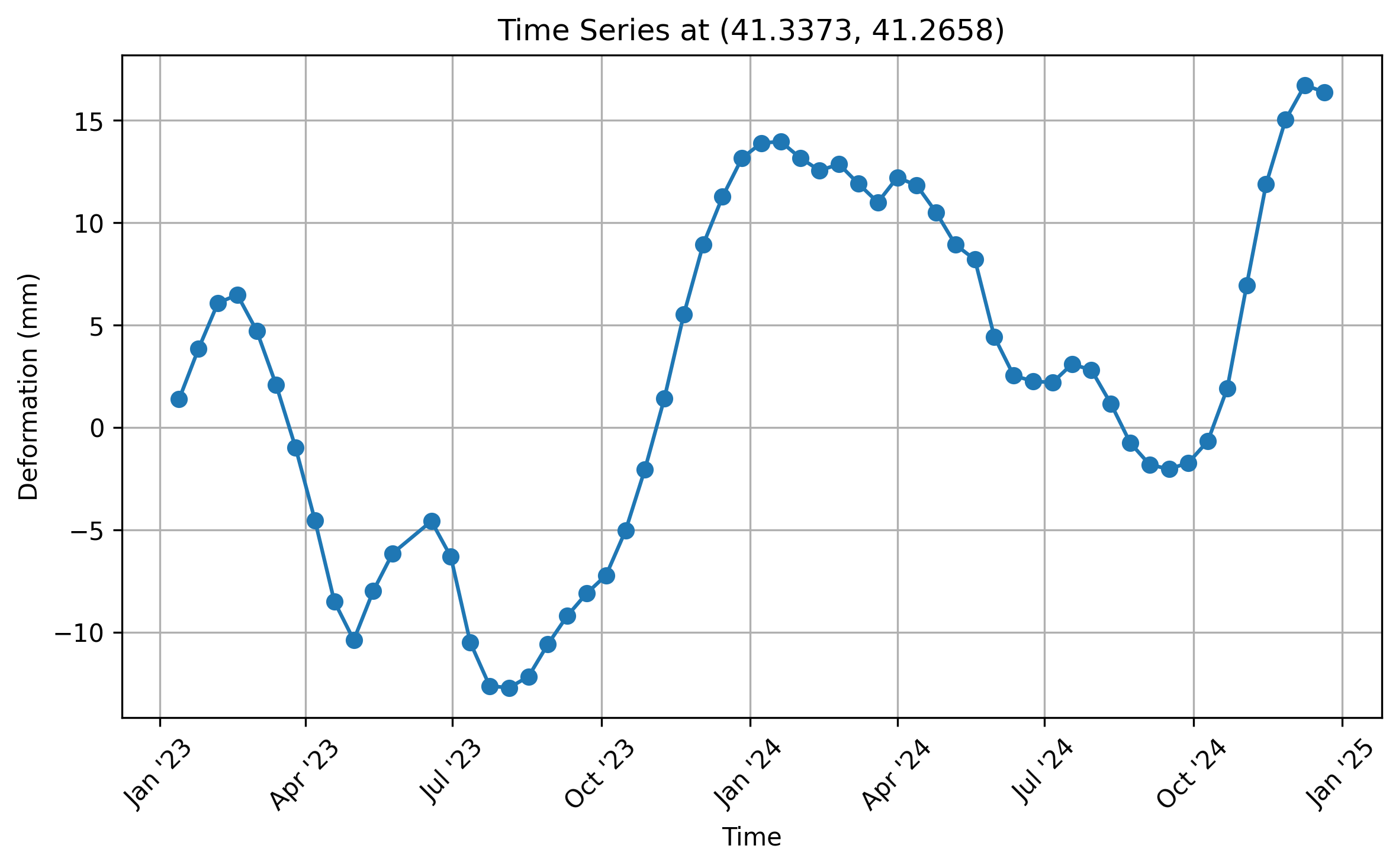
What’s shown: Deformation time series for a pixel near the landslide crown (N41.3373°, E41.2658°).
Plot elements:
X-axis: Time (dates from ~Feb 2023 to Dec 2024)
Y-axis: Line-of-sight displacement (mm)
Blue dots: Individual epoch measurements
Red line: Trend (if fitted)
Key observations:
Steady deformation: Consistent negative trend through 2023
Acceleration: Noticeable increase in deformation rate in November 2024
Pre-failure signal: ~1 month of accelerated deformation before December 8, 2024 failure
Total displacement: ~35-40 mm cumulative LOS displacement
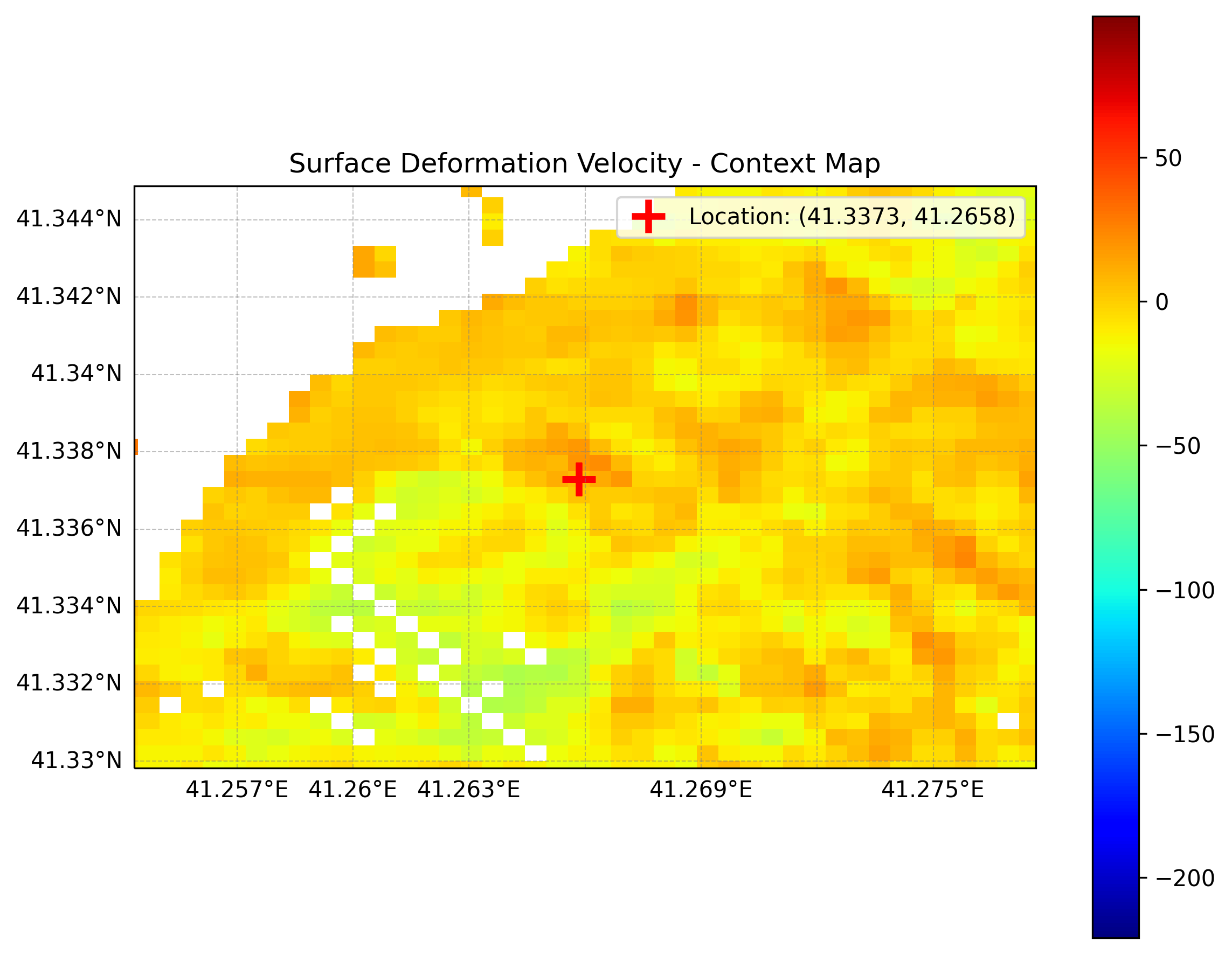
What’s shown: Context map showing pixel location (red dot) on mean velocity background.
Geographic context:
Pixel location relative to deformation pattern
Surrounding velocity field
Landslide extent visible in velocity map
Step 7.2: Deformation Analysis
Mean Annual Velocity:
Line-of-sight velocity (VLOS) reaches up to 25 mm/yr in the source area
Concentrated deformation around landslide crown
Consistent spatial pattern across time series
Time Series Characteristics:
Baseline period (early 2023): Relatively stable or slow deformation
Pre-failure acceleration (November 2024): Measurable increase in deformation rate
Failure event (December 8, 2024): Culmination of progressive slope failure
Post-failure: Data availability pending (may show catastrophic displacement)
Precursory Signal Detected: ✅ InSAR successfully captured the precursory deformation signal approximately one month before the catastrophic failure.
Step 7.3: Scientific Significance
This analysis demonstrates several key capabilities of InSAR and InSARLite:
Landslide Precursor Detection:
InSAR can detect subtle surface deformation (mm-scale precision)
Acceleration patterns visible weeks to months before failure
Potential for early warning applications
Temporal Monitoring:
60 acquisitions over 18 months provide dense temporal sampling
12-day revisit enables detection of rapid changes
Time series reveals progression from stable → slow → accelerated → failure
Spatial Coverage:
Complete coverage of landslide area and surroundings
Identification of most active zones
Context of regional deformation patterns
Validation of InSARLite:
Automated workflow from raw data to scientific results
Publication-quality outputs
Real-world research application
Reference: Gorum et al., 2025 (documentation of Güngören landslide failure)
Part 8: Output Files and Data Products
Step 8.1: Project Directory Structure
After complete processing, your project folder contains the following basic structure:
project_folder/asc/
└── data/
    ├── *.SAFE/                   # Symlinks of Sentinel-1 SAFE directories
    └── S1*.EOF                    # Downloaded precise orbit files
│
│
├── topo/                          # Topographic products
│   └── dem.grd                    # Symlink of DEM in radar coordinates
│
└── F2/                            # IW2 subswath processing
    ├── raw/
    │   ├── *.tiff/                # Symlinks of relevant TIFF files per subswath and user-selected polarization
    │   └── S1*.EOF                # Symlinks for precise orbit files
       ├── 202XXXXX.SLC          # Single Look Complex images
       └── 202XXXXX.PRM          # Parameter files
    ├── baseline_table.dat        # Baseline information
    ├── intf.in                   # Interferogram pair list

    │
    ├── topo/                         # Topographic products
         ├── dem.grd                   # Symlink of DEM in radar coordinates
         ├── trans.dat              # Transformation table for geo-radar coordinates conversion
         ├── topo_ra.grd              # DEM in radar coordinates
         ├── master.prm              # Master metadata file

    │
    ├── intf_all/                 # All interferograms
        ├── corr_stack.grd              # Mean correlation
        ├── std.grd              # Correlation std deviation
    │   └── 2023XXXX_2024XXXX/    # Individual interferogram folders
    │       ├── phasefilt.grd     # Filtered wrapped phase
    │       ├── unwrap.grd        # Unwrapped phase
    │       ├── unwrap_pin.grd   # Normalized unwrapped phase
    │       ├── corr.grd          # Coherence
    │
└── SBAS/                     # Time series results
   ├── disp_YYYYMMDD.grd     # Displacement at each epoch
   ├── vel.grd               # Mean velocity (radar coords)
   ├── vel_ll.grd            # Mean velocity (geographic)
   ├── vel.kml               # Google Earth overlay
   │
   └── time_series/          # Extracted time series
      └── polygon_9vertices_15pixels/
            ├── timeseries_*.png      # Plots (raster)
            ├── timeseries_*.eps      # Plots (vector)
            ├── timeseries_*.pdf      # Plots (vector)
            ├── timeseries_*.svg      # Plots (vector)
            ├── timeseries_*.csv      # Data (for analysis)
            └── timeseries_*_map.png  # Location maps
Step 8.2: Key Output Files
For further analysis:
Velocity map:
SBAS/vel_ll.grd(geographic coordinates)Import into GIS software
Overlay on satellite imagery
Compare with field observations
Time series data:
SBAS/time_series/*/timeseries_*.csvColumns: Date, Displacement (mm), Uncertainty (optional)
Import into Python/MATLAB/R for analysis
Statistical analysis, trend detection, modeling
Displacement grids:
SBAS/disp_YYYYMMDD.grdDisplacement at each epoch
Create animations of deformation evolution
Calculate displacement rates between epochs
Google Earth overlay:
SBAS/vel.kmlOpen in Google Earth
Visualize deformation in 3D context
Share with collaborators
Step 8.3: Export Formats
Time Series:
PNG: Raster image for presentations, quick viewing
EPS: Vector format, publication-ready, scalable
PDF: Vector format, portable, easy sharing
SVG: Vector format, web-friendly, editable
CSV: Raw data for further analysis
Spatial Data:
GRD (GMT): NetCDF format, compatible with GMT, Python (xarray/rasterio)
KML: Google Earth overlay
GeoTIFF: Can be converted using GMT
grd2tifffor GIS use
Part 9: Summary and Next Steps
What You’ve Accomplished
Throughout this tutorial, you’ve completed the entire InSARLite workflow:
✅ Installation (Part 1):
Installed GMTSAR automatically
Configured environment
✅ Project Configuration (Part 2):
Downloaded 60 Sentinel-1 acquisitions
Extracted and validated data
Downloaded and prepared DEM
Configured output structure
✅ Baseline Network (Part 3):
Downloaded precise orbits
Calculated baselines
Selected optimal master (Aug 29, 2023)
Defined network constraints (250m, 48 days)
Generated interferometric pairs
✅ Interferogram Generation (Part 4):
Aligned all images to master
Generated wrapped interferograms
Calculated mean correlation
✅ Phase Unwrapping (Part 5):
Created composite mask (threshold + polygon)
Unwrapped all interferograms
Selected reference point
Normalized phases
✅ SBAS Inversion (Part 6):
Solved for displacement time series
Calculated mean velocity
Launched interactive visualization
✅ Results Analysis (Part 7):
Extracted time series in polygon
Identified precursory deformation signal
Interpreted landslide dynamics
Key Findings
Güngören Landslide Analysis:
Mean VLOS: Up to 25 mm/yr
Precursory acceleration: November 2024 (~1 month before failure)
Failure date: December 8, 2024
Early warning potential demonstrated
Processing Time Summary
Total: ~50+ hours for 60 acquisitions (highly dependent on CPU cores)
Step |
Time |
|---|---|
Installation |
15-30 min |
Data download |
1-3 hours (varies with connection) |
Data extraction |
30-60 min |
Baseline network |
10-15 min |
IFG generation |
30-40 hours (parallel recommended) |
Unwrapping |
8-12 hours |
SBAS inversion |
2-4 hours |
Visualization |
Instant |
Note: Processing times are highly dependent on CPU cores (parallel processing). Single-core processing may take significantly longer.
Best Practices Learned
Master Selection: Use network centrality for optimal connectivity
Baseline Constraints: Balance network density and coherence
Mask Definition: Combine threshold and polygon for optimal unwrapping
Reference Point: Select stable, high-coherence area outside deformation zone
SBAS Parallel: Use all CPU cores for faster inversion
Polygon Analysis: Extract multiple pixels to assess spatial variability
Further Exploration
Additional Analyses:
Process other subswaths:
Include IW1 and IW3 for wider coverage
Merge subswaths for complete swath
Experiment with parameters:
Try different baseline thresholds
Adjust correlation threshold
Compare different reference points
Advanced techniques:
Atmospheric correction (GACOS/tropospheric models)
Ionospheric correction (for longer wavelengths)
2D decomposition (ascending + descending orbits)
Validation:
Compare with GPS data (if available)
Validate with field observations
Compare with other InSAR processors
Time series analysis:
Fit linear/non-linear models
Detect change points
Forecast future deformation (with caution)
Troubleshooting
Common issues and solutions:
Issue |
Solution |
|---|---|
Low coherence |
Adjust baseline constraints, use shorter temporal baselines |
Download failures |
Check Earthdata credentials, internet connection |
Unwrapping errors |
Lower correlation threshold, adjust mask, check reference point |
SBAS convergence |
Increase smoothing, reduce atmospheric iterations |
Memory errors |
Process fewer interferograms at once, use more swap |
Resources
InSARLite:
Documentation: https://insarlite.readthedocs.io
Issues: Report bugs/request features on GitHub
GMTSAR:
Manual: https://topex.ucsd.edu/gmtsar/
Forum: GMTSAR Google Group
Sentinel-1:
Toolbox: https://sentinel.esa.int/web/sentinel/toolboxes/sentinel-1
Data access: https://search.asf.alaska.edu/
InSAR Background:
Ferretti et al. (2007): InSAR Principles
Berardino et al. (2002): SBAS algorithm
Chen & Zebker (2002): Phase unwrapping
Citation
If you use InSARLite in your research, please cite:
[Citation information to be added upon publication]
And acknowledge the data sources:
Sentinel-1 data: ESA Copernicus Programme
SRTM DEM: NASA/USGS
Precise orbits: ESA
Acknowledgments
ESA for Sentinel-1 data and precise orbits
NASA JPL for GMTSAR development
GMTSAR development team for the excellent InSAR processor
InSARLite contributors for tool development and testing
Gorum et al. for Güngören landslide documentation
Conclusion
Congratulations! You’ve successfully completed a comprehensive InSAR time series analysis using InSARLite. You’ve:
Processed 60 Sentinel-1 acquisitions from raw data to scientific results
Detected precursory deformation signals before a catastrophic landslide
Generated publication-quality outputs
Learned the complete InSAR workflow
This analysis demonstrates:
InSAR’s capability for landslide monitoring and early warning
InSARLite’s effectiveness for automated, user-friendly InSAR processing
The importance of dense temporal sampling for capturing rapid deformation
Next steps:
Apply this workflow to your own study areas
Explore advanced processing options
Integrate InSAR with other monitoring techniques
Contribute to InSARLite development
Questions or issues? Open an issue on GitHub or consult the documentation.
Happy InSARing! 🛰️🌍